Ordinary Differential Equations II
In the ODE I tutorial, you learned how to solve ODEs using the Euler and Euler-Cromer methods. You also learned that both these methods are susceptible to truncation error of O(τ2). In this lesson you will learn to use a sophisticated ODE solver called odeint in the scipy.integrate package. It is uses a tried and true ODE solver called lsoda which is part of ODEPACK. ODEPACK is a set of very powerful ODE solvers written by computer scientists at Lawrence Livermore National Lab.
The orbit problem
We will illustrate the use of odeint by using it to determine the orbits of objects—planets, asteroids, comets—orbiting the Sun. Of course, this problem is easily solved analytically. This makes it easy to compare our numerical solution to the correct solution. If they disagree we know there is a problem with our numerical solution. In fact we will find that the Euler method fails spectacularly for the orbit problem.
We will start by reviewing some of the physics of orbits. The gravitational force on a satellite of mass m is
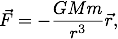 where M is the mass of the Sun, G is Newtonian gravitational constant, and
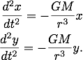
  is the satellite's position vector pointing from the the Sun to the satellite. By Newton's second law the equations of motion for the satellite are
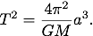
 The solutions are elliptical orbits with the Earth at one focus of the ellipse. The period of the orbit T is related to the semi-major axis a of the ellipse,
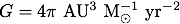
 If we use a system of units where we measure time in years, distance in AU (astronomical units, 1 AU = 1.50 × 10¹¹ m), and masses in multiples of the mass of the sun (
 = 1.99 × 1030 kg) then
 and for the solar system Kepler's third law becomes
  . We will use this convenient system of units in all of the programs below.
The failure of Euler's method
The script below uses Euler's method to solve the orbit problem.
"""
kepler_euler.py
Script to solve the orbit problem using Euler method.
"""

## Import needed modules
from pylab import *
G = 4*pi**2	# define G.

## Set initial position and speed of satellite.
M  = 1.0	# mass of the central mass

# give info to help user decide on initial conditions
Ro = 1.0	# Radius of the orbit
v =sqrt(G*M/Ro)	# v assuming circular orbit
print("For circular orbit of r = %g, and v = %g." % (Ro,v))

# prompt user for initial conditions and times
x0 = input('Initial radius: ')
vy0 = input('Initial tangential velocity: ')
y0 = 0.
vx0 = 0.

t0 = 0.
tf = input("Enter final time: ")
tau = input("Enter time step: ")

## Create arrays needed to store the results for plotting
x_plt = array([x0])
y_plt = array([y0])
vx_plt = array([vx0])
vy_plt = array([vy0])
t_plt = array([t0])

## Execute Euler method
# set starting points for iteration to initial conditions
x_old = x0
y_old = y0
vx = vx0
vy = vy0
t = t0	# set starting time to 0

while (t < tf):
	x = x_old + vx*tau        # implement Euler step
	y = y_old + vy*tau
	r = sqrt(x**2 + y**2)
	vx = vx - tau*(G*M*x)/r**3
	vy = vy - tau*(G*M*y)/r**3

	x_plt = append(x_plt,x)   # Append new points to the arrays
	y_plt = append(y_plt,y)
	vx_plt = append(vx_plt,vx)
	vy_plt = append(vy_plt,vy)
	t_plt = append(t_plt,t)

	x_old = x    # Update x_old and y_old for next Euler step
	y_old = y
	t = t + tau  # Increment time

## Plot the results
figure(1)
clf()

# Plot the orbit
subplot(2,1,1) # subplot() lets you put
               # multiple plots on a single page

title(r'Euler Method with $x$ = %g, $v_y$ = %g, and $\tau$ = %g' \
      % (x0,vy0,tau))
plot(x_plt,y_plt)

centerx = 0.    # plot the position of the center of mass
centery = 0.
plot(centerx,centery,'ko')
axis('equal')   # make axis scales equal so circular orbits look circular

## Plot the energy
subplot(2,1,2)
eps = 0.5*(vx_plt**2 + vy_plt**2) - G*M/sqrt(x_plt**2 + y_plt**2)
plot(t_plt,eps)
eps_plot_min = 1.1*min(eps)
axis([min(t_plt),max(t_plt),eps_plot_min,0])
xlabel('t')
ylabel('E/m')
show()
The code assumes the central mass is at the origin of the coordinates. The initial conditions place the satellite at a user defined distance from the central mass on the x axis. The initial velocity is taken to be perpendicular to the x axis, in the positive y direction. The script also prompts the user for the time step, τ, and the ending time for the computation.
The script plots the orbit as well as the total energy per unit mass as a function of time. We know energy is conserved so this should be a constant. If it isn't we know our algorithm isn't giving good results. The plot below shows the result for the Earth's orbit, r = 1.0 AU, v = 6.3 AU/yr and time steps of τ = 0.01 yr.
The results look reasonable. As expected the orbit is circular and the energy is constant. Download kepler_euler.py and try it for a few different initial conditions. You will find that it doesn't work very well for elliptical orbits. The plots below show that the Euler method fails for r = 1.0 AU, v = 4.0 AU/yr and time steps of τ = 0.01 yr. The orbit isn't closed and the energy isn't conserved.
Exercise 1
Modify kepler_euler.py code to plot the angular momentum per unit mass instead of the energy. Since there are no external torques on the satellite, it's angular momentum should be conserved too. The angular momentum per unit mass for the satellite is
 Run your program for the case r = 1.0 AU, v = 6.3 AU/yr and time steps of τ = 0.01 yr, v = 4.0 AU/yr and time steps of τ = 0.01 yr. Does the Euler method conserve angular momentum?
We clearly need a better algorithm to solve the orbit problem numerically.
Preparations
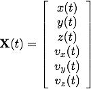
Typically the first step in solving any system of ODEs is to convert them into a system of first-order ODEs. We will approach this step in a very systematic way by writing the system formally as
 where the bold-face type indicates an abstract vector. The vector X(t) is called the state vector. For example, the equations of motion for a particle of mass m under the influence of the force
  are given by Newtons Second Law
  . This defines a system of three second-order ODEs. We can write this system in the state vector notation above by defining
 and
and
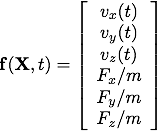 which is a system of six first order ODEs.
Euler's method has a nice compact form when we use the state vector notation

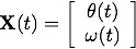
Let's examine a more specific example. For the simple pendulum the equation of motion is the second order differential equation
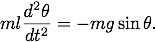 Noting that
  and a little algebra leads to the following two equations
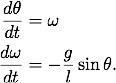 In this case we let
 and
and
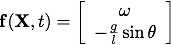 Using the equation
  recovers the system of two first-order equations.
Exercise 2
Determine X and f(X,t) for the following differential equations.
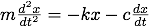
- Damped harmonic oscillator
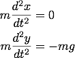
- The trajectory of a particle in two dimensions
- The third order differential equation

Once you think you have the correct equations you can check your work on the ODE II solutions page.
Using odeint()
The odeint() function is part of the scipy.integrate package. It has three required arguments. The first argument is the name of the Python function that defines f(X,t). The second argument is a state vector containing the initial conditions. This state vector is specified as an array. The final argument is an array containing the time points for which to solve the system. The output is a two-dimensional array. It is an array of state vectors for each time point. The first index specifies the time point and the second index specifies the element of the state vector.
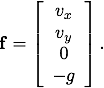
An example will make this clearer. Lets solve problem of a projectile launched launched from ground level at an angle of 45° with a speed of 10.0 m/s. First we convert the equation of motion  into state vector notation. If we let
 then
then
 The code below uses these initial conditions and the definitions of X and f above to solve the trajectory problem.
"""
trajectory.py
"""
import numpy as np
import matplotlib.pyplot as plt
from scipy.integrate import odeint

## set initial conditions and parameters
g = 9.81            # acceleration due to gravity
th = 45.            # set launch angle
th = th * np.pi/180.   # convert launch angle to radians
v0 = 10.0           # set speed

x0=0                # specify initial conditions
y0=0
vx0 = v0*np.cos(th)
vy0 = v0*np.sin(th)

## define function to compute f(X,t)
def f_func(state,time):
    f = np.zeros(4)    # create array to hold f vector
    f[0] = state[2] # f[0] = x component of velocity
    f[1] = state[3] # f[1] = x component of velocity
    f[2] = 0        # f[2] = acceleration in x direction
    f[3] = -g       # f[3] = acceleration in y direction
    return f

## set initial state vector and time array
X0 = [ x0, y0, vx0, vy0]        # set initial state of the system
t0 = 0.
tf_str = input("Enter final time: ")
tau_str = input("Enter time step: ")
tf = float(tf_str)
tau = float(tau_str)

# create time array starting at t0, ending at tf with a spacing tau
t = np.arange(t0,tf,tau)

## solve ODE using odeint
X = odeint(f_func,X0,t) # returns an 2-dimensional array with the
                        # first index specifying the time and the
                        # second index specifying the component of
                        # the state vector

# putting ':' as an index specifies all of the elements for
# that index so x, y, vx, and vy are arrays at times specified
# in the time array
x = X[:,0]
y = X[:,1]
vx = X[:,2]
vy = X[:,3]

## plot the trajectory
plt.figure(1)
plt.clf()

plt.plot(x,y)
plt.xlabel('x')
plt.ylabel('y')
plt.show()
Notice that odeint(f_func,X0,t) takes three arguments as input. The first is the name of a function that returns the vector f. When odeint() runs it calls the function f_func(state,time) and expects its two input arguments be in a certain order and be of a certain type. The first argument must be an numpy array specifying a state vector. The second argument must be a float that specifies the time. Odeint() also requires that f_func() return an array containing the value of f evaluated for the given input state and time. If the input and outputs of f_func() don't have the correct type, odeint() won't run. This is why we must specify a time input argument in f_func() even though our particular system of equations doesn't depend explicitly on time.
Running the trajectory.py program with an ending time of 1.44 s and time steps tau = 0.01 s gives the plot shown below.
This is just what we expect for the trajectory of the projectile.
Exercise 3
Modify trajectory.py to add a drag force  . Take k = 0.22 kg/m and m = 5 kg. Plot the trajectory and the energy. Does the energy do what you expected? Where does the energy go?
The orbit problem revisited
The program kepler.py is a modified version of trajectory.py that solves the orbit problem using odeint(). Examine the code below and make sure you understand how it works.
"""
kepler.py
Script to solve the orbit problem using the scipy.integrate.odeint().
"""

## Import needed modules
from pylab import *
from scipy.integrate import odeint
G = 4*pi**2 # define G for convenience.

## Set initial position and speed of satellite.
# Compute and display some values for a circular orbit to help decide
# on initial conditions.
Ro = 1.0    # Radius of the orbit
M  = 1.0    # mass of the central mass

v =sqrt(G*M/Ro) # v assuming circular orbit

# Get initial position and speed.
print("For circular orbit of r = %g, and v = %g." % (Ro,v))
x0 = input('Initial radius: ')
vy0 = input('Initial tangential velocity: ')

## Set initial conditions and define needed array.
X0 = [ x0, 0, 0, vy0]       # set initial state of the system
t0 = 0.
tf = input("Enter final time: ")
tau = input("Enter time step: ")
t = arange(t0,tf,tau)   # create time array starting at t0,
                        # ending at tf with a spacing tau

## Define function to return f(X,t)
def f_func(state,time):
    f=zeros(4)
    f[0] = state[2]
    f[1] = state[3]
    r = sqrt(state[0]**2 + state[1]**2)
    f[2] = -(G*M*state[0])/r**3
    f[3] = -(G*M*state[1])/r**3
    return f

## Solve the ODE with odeint
X = odeint(f_func,X0,t) # returns an 2-dimensional array with
                        # the first index specifying the time
                        # and the second index specifying the
                        # component of the state vector

x = X[:,0]  # Giving a ':' as the index specifies all of the
            # elements for that index so
y = X[:,1]  # x, y, vx, and vy are arrays that specify their
vx = X[:,2] # values at any given time index
vy = X[:,3]

## Plot the results
figure(1)
clf()

# Plot the orbit
subplot(2,1,1)
title(r'Using odeint with $x$ = %g, $v_y$ = %g, and $\tau$ = %g' \
      % (x0,vy0,tau))
plot(x,y)
centerx = 0.
centery = 0.
plot(centerx,centery,'ko')
axis('equal')

# Plot the energy
subplot(2,1,2)
eps = 0.5*(vx**2 + vy**2) - G*M/sqrt(x**2 + y**2)
plot(t,eps)
eps_plot_min = 1.1*min(eps)
axis([min(t),max(t),eps_plot_min,0])
xlabel('t')
ylabel('E/m')
show()
Running kepler.py with r = 1.0 AU, v = 4.0 AU/yr and time steps of tau = 0.01 yr gives the result below.
These are the same conditions as specified for the example in which the Euler method failed. Odeint() gives correct results for the same conditions. It's fast and it gives better results so there is no reason not to use it to solve ODEs unless there is some special application that odeint() can't accommodate.
Exercise 4
Try kepler.py with other initial conditions for which you know the result. Can you make if fail? If so, can you get better results with a smaller time step?