Ordinary Differential Equations I
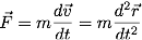
The theoretical foundations of mechanics are Newton's three laws. Newton's second law,  essentially defines a set of three coupled second-order ordinary differential equations (ODEs). Let
  be the position vector and
  the velocity vector of some mass m then the second law is
 or in cartesian coordinates
 If we solve this system of ODEs with the initial conditions
  and
and  we know all there is to know about the particle's motion.
Euler's Method
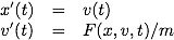
Let's first consider motion in one dimension. In the x-direction Newton's second law give a second-order differential equation x''(t) = F(x,v,t)/m where the prime indicates differentiation with respect to time. To get the motion of the particle we need to find x(t). The first step in solving ODEs numerically is to convert the second order equation into two first-order equations
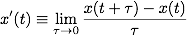
 Now we need some way to numerically evaluate derivatives. Recall the formal definition of a derivative
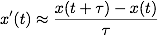
 We can numerically approximate a derivative by using some very small but finite value of τ
 If we rearrange this equation and note that x'(t) = v(t) we get
 We can find v(t + τ) using the same method on the first-order equation for v'(t),
 this suggests an iterative method for finding x(t) and v(t). Starting with the known initial conditions x(0) and v(0) we can compute v(τ) using the equation above. We then use this to find x(τ). We now use these values and repeat the process to generate x and v for all the time we desire. This method of solving ODEs is called Euler's Method.
Galileo's Problem
Let's illustrate Euler's Method by solving for the postion and speed of an object dropped from a height. Galileo is reputed to have done this with two objects with different masses. Galileo reported that both objects hit the ground at the same time, thus establishing that the force of gravity near the surface of the Earth was Fg = -mg. We will start by solving this problem without taking into account air resistance. Of course we can do this without a computer, but it will be a nice test of Euler's Method and be a good starting point for solving the problem with air resistance.
Before we start let's write the equations of Euler's Method in a form that is a little easier to translate to code. As we step through Euler's method we will generate a set of x and v values at a discrete set of times tn = nτ for n = 0, 1, 2,... . Let xn = x(tn), and vn = v(tn). Note also that the acceleration a(x,v,t) = F(x,v,t)/m so define an = a(xn,vn,tn) = F(xn,vn,tn)/m. The equations for Euler's Method in our new notation are
| vn+1 | = | vn + anτ |
| xn+1 | = | xn + vnτ. |
The code below takes as inputs the initial height (y0), and the size of the time step. It then solves for y and v as a function of time using Euler's method assuming v0 = 0. It assumes the force is F = -mg or a = -g. Finally, it plots y as a function of time along with a plot of the result using the kinematics equations for comparison.
"""
galileo.py
Program to compute the position of an object dropped from a height y0 using
Euler's method and compare it to the result using kinematics.
"""

## Import needed modules

from pylab import *
import scipy.constants as pc

## Prompt user for inputs

y0_str = input("Starting height (m): ")
y0 = float(y0_str)
tau_str = input("Size of the time steps (s): ")
tau = float(tau_str)

## Solve for y and v using Euler's method

y_old = y0	# Set the initial values of y, v, and t
v = 0.0
t = 0.0

y_plt = array([y_old])	# Create arrays to record the position, velocity,
                        # and time for plotting
v_plt = array([v])
t_plt = array([t])

while (y_old > 0):
	y = y_old + v*tau	# Euler step to compute y
	a = -pc.g		# Compute the acceleration from the force
	v = v + a*tau	# Euler step to compute v

	y_old = y		# set the position for the next iteration
	t = t + tau		# Increment the time

	y_plt = append(y_plt,y) # Append new points to the plotting arrays
	v_plt = append(v_plt,v)
	t_plt = append(t_plt,t)

## Use kinematics equations to compute the comparison y and v
y_k = y0-pc.g*t_plt**2/2.
v_k = -pc.g*t_plt

## Plot height as a function of time
figure(1)
clf()
plot(t_plt,y_plt,'r+',label="Euler's method")
plot(t_plt,y_k,'k-',label="Kinematics equations")
legend()
xlabel('time (s)')
ylabel('height (m)')

## Plot the velocity as a function of time
figure(2)
clf()

plot(t_plt,v_plt,'r+',label="Euler's method")
plot(t_plt,v_k,'k-',label="Kinematics equations")
legend()
xlabel('time (s)')
ylabel('velocity (m/s)')
show()

## Print time of flight and final speed
print("\nTime of flight is %g sec." % t)
print("Speed at impact is %g m/s." % v)
With an initial height of 100 m and a time step τ = 0.1 seconds the program gives the plot shown below. Euler's method does a good job of approximating the correct trajectory. We will soon see this isn't always the case.
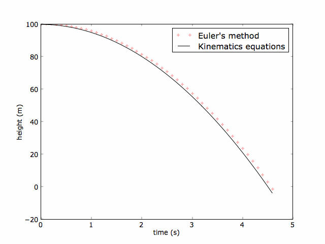
The time of flight computed in the above example is 4.5 seconds. Can you improve the accuracy by using a smaller time step? Try it and see if Euler's method still gives a good result. Is there a limit to how small you can choose the time step? You might get tired of waiting. There are faster methods we will deal with in the ODE II tutorial. If you are patient, you will find there is a limit. Round-off error will destroy the accuracy of the result if the time step is too small. The tutorial on Computation Errors has a more complete discussion. For a short discussion of some real-life examples of round-off error see the Roundoff Error article on the Wolfram site.
Exercise 1
The goal of this exercise is to modify the galileo.py program to take into account air resistance. Air resistance depends on the shape, size, and speed of the falling object. For objects moving through air the drag force can be approximated as
 where v is the speed of the object,
  is a unit vector in the direction of the velocity, ρ is the density of air, A is the cross-sectional area of the object, and Cd is the drag coefficient. The drag coefficient is dimensionless and depends on the shape of object. For a smooth spherical object moving faster than about 0.2 m/s Cd ≈ 0.5. If the drag force is included then the object's motion does depend on its mass.
Modify the galileo.py program to account for the drag force. Use this to compute the time of flight for two different spherical masses of the same dimensions falling from a height of 100 m. Assume the masses are 100 kg and 1 kg, and that the radius of both masses is 15 cm. Take the density of air to be 1.2 kg/m3.
Simple Pendulum
Galileo was also the first to recognize that the for small oscillations, the period T of a simple pendulum depends only on its length,
 where l is the distance from the pivot to the mass and g is the acceleration due to gravity. On the Numerical Integration Toolbox page you can see how to compute the period when the amplitude is large, but what if we want to determine the angular displacement of the pendulum θ(t) given some initial conditions θ0 and ω0. For large amplitudes this motion is no longer sinusoidal. To determine the angular displacement we must solve the differential equation
 (see any mechanics book for the derivation).
We can't solve this equation analytically, but we can numerically. The first step is to, again, convert this second-order differential equation into two coupled first-order equations
 The corresponding Euler steps are
| ωn+1 | = | ωn - (g / l) sin(θn)τ |
| θn+1 | = | θn + ωnτ. |
The code below implements Euler's method to solve the simple pendulum problem.
"""
pendulum.py
Program to compute the angular displacement and angular velocity for a simple
pendulum using Euler's method.
"""

## Import needed modules

from pylab import *
import scipy.constants as pc


## Set initial conditions

th0 = float(input("Starting position for pendulum in degrees: "))
th0 = th0 * pi/180.	# Convert starting angle to radians
om0 = 0.0
l = 10.				# Length of pendulum in m

T_est = 2*pi*sqrt(l/pc.g)
print("Estimated period is %g s " % T_est)

N_period = float(input("Approximate number of periods to plot: "))
t_max = N_period * T_est

tau = float(input("Size of the time step (s): "))

## Solve ODE using Euler's method

th_old = th0	# Set the initial values of angular displacement, angular
                # velocity, and t (time).
om = om0
t = 0.0

th_plot = array([th_old]) # Make arrays to record the th, om, and t for plotting
om_plot = array([om])
t_plot = array([t])

while (t < t_max):
	th = th_old + om * tau					# first Euler step
	om = om - pc.g/l * sin(th_old) * tau	# second Euler step

	th_old = th	# set the angle for the next iteration
	t = t + tau	# increase the time by one time step

	th_plot = append(th_plot,th)	# append this step's result to the plotting
	                                # arrays
	om_plot = append(om_plot,om)
	t_plot = append(t_plot,t)

th_plot = th_plot*180./pi	# Convert angle back to degrees

## Plot the results
figure(1)
clf()
plot(t_plot,th_plot,'r+')
xlabel('time (seconds)')
ylabel(r'$\theta$ (degrees)')
show()
It is a good idea to check your programs with a simple case for which you know the solution. Let's check the program with small a small oscillation of 10° and a pendulum of length 10 m. This is a long pendulum, but not out of the question for one of the chandeliers that Galileo may have watched in a cathedral in Venice. The result is shown below for a step size of 0.1 seconds.
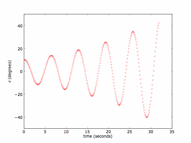
Clearly, the Euler method isn't working in this case. The amplitude and hence the energy of the pendulum is growing as time goes on. The Euler method would give better results for smaller time steps, but would take longer. The problem is results from truncation error.
Exercise 2
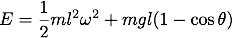
Modify pendulum.py to also plot the energy per unit mass of the pendulum as a function of time. Recall that if we take the potential energy of the mass to be zero at the bottom of the swing then the total energy for the pendulum is
 Run your program with time steps of 0.1, 0.01, and 0.001 seconds for approximately five periods. By what fraction does the energy change given these three time steps? Did the result improve with smaller time steps? Did the program take significantly longer for the smaller time steps?
Truncation Error
Truncation error occurs because we are approximating the infinitesimal dt by a small, but finite time step τ. We can quantify the truncation error by expanding x(t) in a Taylor series about t
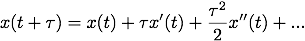 The first two terms in the equation above are the same as the approximation derived from the forward derivative above. The τ2 term is the next largest term in the series and is an approximation of the truncation error. Sometimes you will see the above equation written
 which indicates that the truncation error is of order τ2. Of course the we can make the truncation error smaller by picking a smaller τ, but we pay the price in increased computing time. A better alternative would be to find another way to approximate derivatives where the truncation error depends on a higher power of τ.
The truncation error made in a single step of a program is called the local truncation error. The problem with the pendulum problem is that the truncation error in one step contributes to the error in the next step. The overall truncation error is referred to as global truncation error. In some cases a simple change in the code can substantially reduce the global truncation error. For example, a slight modification of Euler method is called the Euler-Cromer method and can significantly reduce the global truncation error in the pendulum problem. The Euler-Comer method uses the updated velocity at each step to compute the position
| vn+1 | = | vn + anτ |
| xn+1 | = | xn + vn+1τ. |
This slight change significantly improves the results for the pendulum problem.
Exercise 3
Modify the program you wrote in Exercise 2 to use the Euler-Cromer method. Try your program with a time step of 0.1 seconds and approximately five periods. By what fraction does the energy change? How does this compare with your results from Exercise 2 using the Euler method.
Run your program with 10° and 179°. How does the shape of the shape of the oscillation change for the larger amplitude?
In the ODE II tutorial we will explore using a much more sophisticated algoritm to solve ODEs using a sophisticated ODE solver in the SciPy package. It's fast an almost always works.