Numerical Integration
For small oscillations, a simple plane pendulum has a period
 where l is the distance from the pivot to the mass and g is the acceleration due to gravity. However, if the amplitude is large then the period is given by an ellipic integral of the first kind
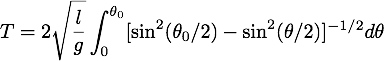 where θ0 is the amplitude of the oscillations. This integral has to be solved numerically. There is no closed form solution.
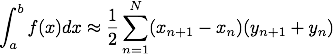
The brute-force way to approximate an integral is replace it by a sum
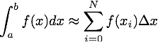 where Δx = (b-a)/N, but there is a better way. We can use a function called
 quad(func,a,b) in the scipy.integrate module. It's better because it's more accurate and faster. The code below numerically integrates the function f(x) = exp(-x3) from 1 to 3.
In [1]: from pylab import *

In [2]: from scipy.integrate import quad

In [3]: def func(x):
   ...:     return exp(-x**3)
   ...:

In [4]: ansr = quad(func,1,3)

In [5]: ansr
Out[5]: (0.085468329429509785, 3.155037254924254e-09)

In [6]: ansr[0]
Out[6]: 0.085468329429509785
The ansr is returned as a tuple of two numbers. (A tuple is kind of like a list, if you really want to understand tuples see the Python documentation on tuples). You access the elements of a tuple like a list. In this case, ansr[0] is the first element of the tuple. The first element of the tuple returned by quad() is the numerical value of the integral, the second is an estimate of the absolute error in the result.
Exercise 1
Numerically integrate the equation for the period of a pendulum for a an amplitude θ0 = π/4. Assume the length of the pendulum is 0.5 m. By how much does this answer differ from the approximate result?
Suppose you now wanted to find the period for a different amplitude, θ0 = π/2 for example. This would require you to modify not only the upper limit of integration, but also the function you integrate because it depends on on the amplitude as well. One way to handle this would be to add another parameter to the argument list of the function that you are integrating. The problem with this is that quad() wouldn't know which argument to integrate over. However, quad() takes the optional argument called args that is a tuple of arguments that are passed on to the integrand function passed to quad(). This sounds complicated, but its easy to implement.
The following example code illustrates how to use the args parameter, the script computes the integral of the function f(x) = α exp(-αx3) from x = 1 to 3, for 0 < α < 1. The value of the integral is plotted as a function of α.
"""
quad_demo.py
Demonstrates using the arg parameter to
pass parameters to the integrand function
when using the quad() function.
"""

# import the needed modules
from pylab import *
from scipy.integrate import quad

# define the integrand function
def func(x, alpha):
	return alpha*exp(-alpha*x**3)

# set the parameters
a = 1   # lower limit of integration
b = 3   # upper limit of integration
N = 100 # number of alpha values to use in integrations

alpha_ary = linspace(0,1,N) # create an array of values of alpha
value = zeros(N)            # create an array to store results of integrations

# do the integrations
idx = 0
for alpha in alpha_ary:
    value[idx],error = quad(func,a,b,args=alpha) # note use of the args optional argument
    idx = idx + 1

# plot the result
figure(1)
clf()
plot(alpha_ary,value)

# note the new syntax for the xlabel() and title() commands
# that allows the use of LaTeX commands
xlabel(r'$\alpha$')
ylabel('Integral')
title(r"Plot of $\int^3_1 \alpha \exp(-\alpha x^3) dx$")
This script generated the plot below. In order to pass a single argument through quad() to the integrand function, we simply have to define the integrand function with a new parameter, func(x, alpha). We pass the alpha parameter through quad() by using its optional args parameter, quad(func,a,b,args=alpha).
The only possible surprise in the code for quad_demp.py is the new syntax in the xlabel() and title() commands. Pre-appending an r before the quoted string in any of the plotting text commands allows you to use LaTeX mathematical formatting commands in the string. Check the Plotting page for details.
Exercise 2
Write a script to plot the period of a plane pendulum as a function of amplitude from 0 to π. Include a line showing the approximate solution for comparison. At what amplitude does the exact solution differ from the approximate solution by 1%?
The SciPy integration routines allow infinite limits of integration, just enter -inf or inf for the limits. Here's an example.
In [1]: from pylab import *

In [2]: from scipy.integrate import quad

In [3]: def gaus(x):
   ...:     return exp(-x**2)
   ...:

In [4]: quad(gaus,-inf,inf)
Out[6]: (1.7724538509055157, 1.4202637044742729e-08)
Exercise 3
In statistics the complementary error function is defined as
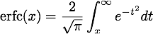
Write a function to compute erfc(x) and a script to plot it from x = -3 to 3.
scipy.stats package, but write your own function for this exercise.
Double and triple integrals
You can compute double and triple integrals with the functions dblquad() and tplquad(). Double and triple integrals are complicated by the fact that the inner limits of integration can depend on the outer integral variable. For example, suppose you need to compute the position of center of mass of the thin triangular plate shown below.
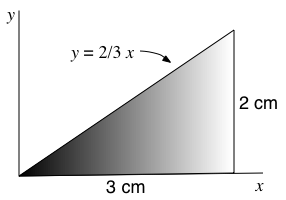
The surface density of the plate is σ(x,y) = 1.3 exp(-x2) gm cm-2. The x and y postion of the center of mass is given by
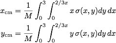 where
where
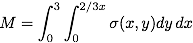 is the total mass of the plate. The upper limit of integration of the inner y integral is given is a function of x; y = 2/3 x. The
 dblquad() function allows you to enter a function for the limits of integration of the inner integrals. The syntax for calling dblquad() is
value, error = dblquad(func, a, b, gfun, hfun, args=(func_params))
where value is the value of the integral, error is the estimated error, func is the integrand, a is the lower limit, and b the upper limit of the outer integration. The next two arguments are functions and specify the lower limit (gfun) and upper limits (hfun) for the inner integration. Unfortunately, you cannot simply enter numbers instead of function for gfun and hfun. Finally, args is the optional parameter for passing values to the integrand as illustrated above for quad().
As an example, lets compute the mass of the plate described above.
"""
dblquad_demo.py
This script computes the total mass of the plate described on the Numerical
Integration webpage.
"""

# import needed libraries
from pylab import *
from scipy.integrate import dblquad

# define functions
# integrand
def sigma(y,x):            # NOTE ORDER OF ARGUMENTS! Required order for dblquad()
    return 1.3*exp(-x**2)  # gm cm^-3, doesn't actually depend on y

# lower limit of y integration
def ylower(x):             # just returns the constant value of 0
    return 0.

# upper limit of y integration
def yupper(x):
    return 2.*x/3.

# compute mass and display result
mass, error = dblquad(sigma,0.,3.,ylower,yupper)

print('The mass of the plate is %g grams' % mass)
The result is M = 0.43328 grams.
Exercise 4
Use dblquad() to determine xcm and ycm of the triangular plate described above.
The syntax for tplquad() is very similar to dblquad(),
value,error = tplquad(func, a, b, gfun, hfun, qfun, rfun, args=(func_params))
It computes the triple integral of func(z,y,x,*args) for x = a to b, y = gfun(x) to hfun(x), and z = qfun(x,y) to rfun(x,y) (args is optional).
Integration of functions given at discrete points
It is common in experimental and numerical work to have measured or computed some function f(x) at a set of discrete values of x, but you need to compute the integral of f(x). In this case you have two arrays, yi = f(xi) and xi and you wish to approximate the integral. The figure below shows an example of a function f(x) (green line), that has been measured at several discrete points yi = f(xi) (blue dots). The total area of the black trapezoids is a good approximation to integral of f(x) from a = 0 to b = 6.28.
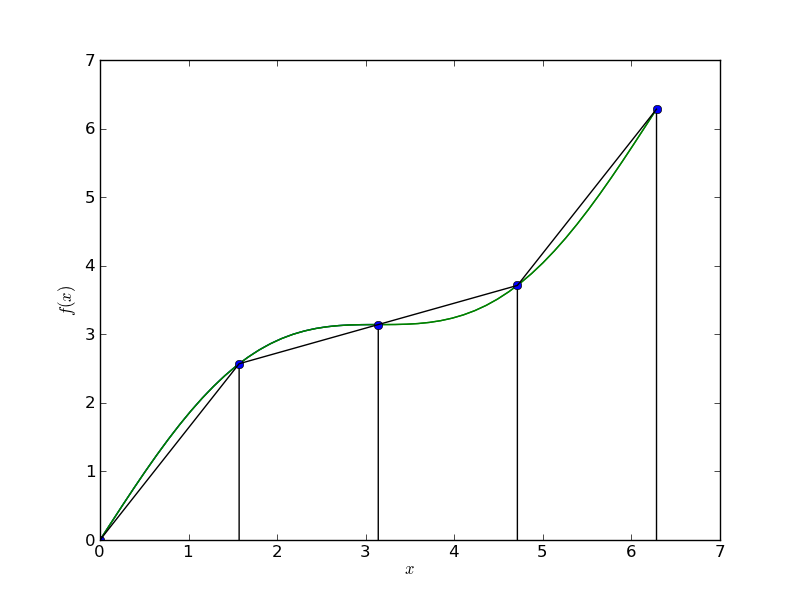
Approximating the integral in this way is called the trapezoidal rule. It's easy to show that the trapezoidal rule is given by the equation
 PyLab has a function for computing discrete integrals called
 trapz(y,x). Note the inverted order of the arguments. The second argument is x and the first argument is y = f(x). The example below illustrates how to use it with the data
xi = {0, 1.57, 3.14, 4.71, 6.28} and yi = {0, 2.57, 3.14, 3.71, 6.28}.
In [31]: from pylab import *

In [32]: xd = array([0.0,  1.57,  3.14,  4.71,  6.28])

In [33]: yd = array([0,  2.57,  3.14,  3.71,  6.28])

In [34]: trapz(yd,xd)
Out[34]: 19.719200000000001
You can learn more about using trapz(y,x) from the
SciPy Documentation.
Exercise 5
An inertial navigation system (INS) uses accelerometers to measure acceleration and then integrates the measured accelerations to determine velocity and position. INS are used in everything from airliners to sensors in running shoes to keep track of distance and speed.
The Downloads page contains a data file called acceleration_data.txt. It contains the acceleration data from an INS system carried by a race car. Use trapz(y,x) to integrate this data to get a plots of the cars speed and position as a function of time. The data starts with the care already traveling at a speed of 1.28 m/s. How does your estimate of the total distance traveled compare to measured distance of 91.5 m?