Data Fitting
One of the most common data analysis problems is fitting a curve to a set of data points. Suppose you have a set of N data points {xi, yi} and that you wish to fit the data to a function y(x) = y(x; a1…aM), where the {ai} are adjustable parameters that give the "best fit." How do we define the "best fit"? We have many choices, but one of the most intuitive is to minimize the sum of the squares of the difference between the data points and the function. In other words, we wish to find the values of {ai} that minimizes the function
 This is called a least-squares fit and is exactly what the
 polyfit() function that we met in the Quick Tour tutorial uses. We used it to find the acceleration due to gravity from some data. Here is the code.
"""
findg.py
Program to determine the acceleration due to gravity from distance
and time data
"""
from pylab import *

## Read the data from the file
t,d = loadtxt('FreeFallData.txt', unpack=True)

## Plot the data and label the graph
plot(t,d,'bo')
xlabel('time (s)')
ylabel('distance (m)')

## Fit a polynomial to the data
(a2,a1,a0) = polyfit(t,d,2)
d_plot = a2*t**2 + a1*t + a0
plot(t,d_plot,'r-')

## Print out the value of g from the fit
g = 2.*a2
print("the acceleration due to gravity is:")
print(g)
This worked well in that it gave us a value for g, but it has a couple of drawbacks. One is that it only works if the fitting function is a polynomial. A more serious drawback for doing experimental work is that it doesn't handle uncertainties. It doesn't give uncertainties in the fit parameters, nor does it take uncertainties in the data points into account.
Using curve_fit()
The scipy.optimize module has just what we need to fit any function and it returns uncertainties in the fit parameters. Not surprisingly, the function is called curve_fit(func,x,y) and it has three required arguments. The first argument func specifies the function to which the data is fit. The second and third arguments specify the data arrays. The interactive session below shows a simple example.
In [10]: from scipy.optimize import curve_fit

In [11]: x=array([1,2,3,4])

In [12]: y=array([0.9,2.1,2.9,4.1])

In [13]: def func(x,a0,a1):
   ....:     return a0 + a1*x
   ....:

In [14]: a_fit,cov=curve_fit(func,x,y)

In [15]: a_fit
Out[15]: array([-0.09999999,  1.04      ])

In [16]: cov
Out[16]:
array([[ 0.02400001, -0.008     ],
       [-0.008     ,  0.0032    ]])
Line 10 imports curve_fit(). Lines 11 and 12 create the data arrays. In this case y = x. I've included a little scatter in the y data points to represent some uncertainty. Line 13 defines the function to which the data should be fit. In this case the fitting function is a straight line with with an intercept a0 and a slope a1. Line 47 defines our best guess for these parameters. Line 14 calls curve_fit(). Curve_fit() returns the two arrays; a_fit contains the best estimates of the fit parameters, and cov holds the covariance matrix. Line 49 displays the best estimate of the fitting parameters. These are just what we expected—the slope is about 1.0 and the intercept is about 0.0. Line 16 displays the covariance matrix. The covariance matrix is a two-dimensional array. The diagonal elements of this array give the variance or square of the uncertainties of the best fit parameters. For example, the uncertainty in the slope is sqrt(cov[1][1]). The best fit slope is therefore 1.04 ± 0.06 and the best fit intercept is -0.10 ± 0.15. These results are consistent with the expected values of 1.0 and 0.0 for the slope and intercept.
Exercise 1
Modify findg.py to use curve_fit() instead of polyfit(). Be sure to display the uncertainty in the in g as well as the best fit value. Verify that both programs gives the same result for g.
Run your new program again, but this time using the data file FreeFallData_err.txt. This file includes some scatter in the measured values of distance which should give larger values for the uncertainty in g.
You can get all of the needed data files from the Downloads page.
So far we haven't taken advantage of the full power of curve_fit(). We have just used it to do exactly the same calculation that is done by polyfit() although we do now get uncertainties in the fit parameters. Let's give it a more difficult task—that of fitting a sinusoid.
The file signal_data.txt contains some noisy data (voltage from an amplifier) that seems to be sinusoidal. (You can download the file from the Downloads page.) Let's try to fit a sinusoidal function of the form V = A sin(2π f t - φ) to these data. In this case the fitting parameters are the amplitude (A), frequency (f ), and phase (φ) of the wave. The interactive session below attempts a fit and plots the result.
In [77]: t,V = loadtxt('signal_data.txt', unpack=True)

In [78]: def fit_func(t,A,f,phi):
   ....:     return A*sin(2*pi*f*t - phi)
   ....:

In [79]: a_fit, cov = curve_fit(fit_func,t,V)

In [80]: plot(t,V,'+r')
Out[80]: [<matplotlib.lines.Line2D object at 0x59ed730>]

In [81]: V_fit = a_fit[0]*sin(2*pi*a_fit[1]*t - a_fit[2])

In [82]: plot(t,V_fit)
Out[82]: [<matplotlib.lines.Line2D object at 0x59ed6b0>]
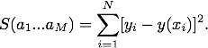
Here's the output plot.
The fit clearly failed! It failed because the Levenberg–Marquardt algorithm that curve_fit() uses needs a "best guess" at the fit parameters as a starting point for its search for the solution that minimizes S(a1…aM). If curve_fit() finds a local minimum in S(a1…aM) it stops searching and hence may miss a global minimum which is a better fit. This is what happened for this set of data points. If no best guess is given to curve_fit() it uses default values equal to 1.0 for all the fit parameters.
The program signal_fit.py tries to remedy this problem by first plotting the data and allowing the user to enter guesses for the fit parameters. It then calls curve_fit(), plots the resulting fit and prints the best estimates of the fit parameters.
"""
signal_fit.py fits a sinusoidal function of the form
V = A*sin(2*pi*f*t - phi) to data using curve_fit(). A,
f, and phi are the fit parameters.
"""
## Import needed modules
from pylab import *
from scipy.optimize import curve_fit

## Read data from the data file
filename = raw_input('File name: ')
t,V = loadtxt(filename, unpack=True)

## Plot the data and allow user to input best guess parameters
figure(1)
clf()
plot(t,V,'+r')
xlabel('t')
ylabel('V')
show()

A_g = input('Estimated amplitude: ')
f_g = input('Estimated frequency: ')
phi_g = input('Estimated phase: ')

a_guess = [A_g,f_g,phi_g]

## Do the fit and decode the output
# Define fit_func
def fit_func(t,A,f,phi):
	return A*sin(2*pi*f*t - phi)

a_fit, cov = curve_fit(fit_func,t,V,p0=a_guess)
A_fit = a_fit[0]
f_fit = a_fit[1]
phi_fit = a_fit[2]

sig_A = sqrt(cov[0][0])
sig_f = sqrt(cov[1][1])
sig_phi = sqrt(cov[2][2])

## Display the results
print('A = %g +/- %g' % (A_fit,sig_A))
print('f = %g +/- %g' % (f_fit,sig_f))
print('phi = %g +/- %g' % (phi_fit,sig_phi))

V_fit = fit_func(t,A_fit,f_fit,phi_fit)
plot(t,V_fit)
show()
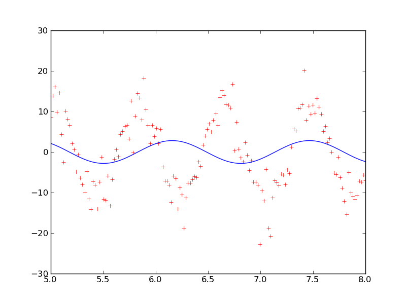
With reasonable values for the best guesses of A = 11.0, f = 1.25, and φ = 0.0, signal_fit.py gives the following plot.
This plot looks like it is giving a good fit. The best fit parameters are A = 11.7 ± 0.4, f = 1.227 ± 0.007, and φ = -3.7 ± 0.3.
Exercise 2
Use signal_fit.py to fit the files signal1.txt and signal2.txt. What are the best fit parameters? Include uncertainties. Do you get good fits? What happens if you give poor guesses for the parameters?
Handling data uncertainties
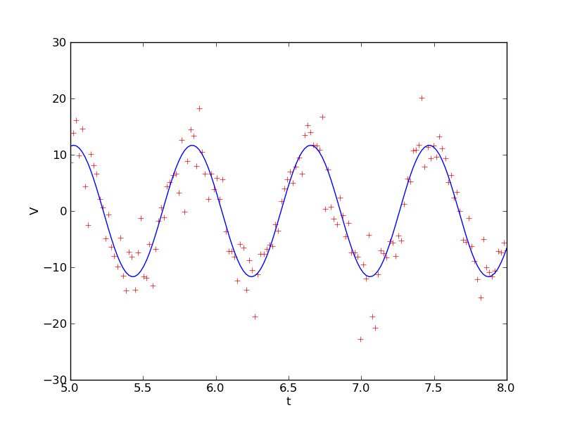
Often you will have estimates of the uncertainties in each of the data points. If some of the data points have small uncertainties and others large uncertainties, the points with large uncertainties can bias the fit. Let's illustrate this with an example. The file Outlier.txt contains x and y data points in the first and second columns along with an error in the y data points in the third column. You can plot the data and show the error bars with the function errorbar(x, y, yerr=sigma). The plot is shown below.
It looks like there is a linear relation between x and y. The session below fits these data and then plots the fit.
In [1]: from scipy.optimize import curve_fit

In [2]: x,y,sigy=loadtxt('Outlier.txt',unpack=True)

In [3]: errorbar(x,y,yerr=sigy,fmt='ro')
Out[3]:
(<matplotlib.lines.Line2D object at 0x5b938d0>,
 [<matplotlib.lines.Line2D object at 0x5b93590>,
  <matplotlib.lines.Line2D object at 0x5b93650>],
 [<matplotlib.collections.LineCollection object at 0x5b84fd0>])

In [4]: def func(func,a,b):
   ...:     return a + b*x
   ...:

In [5]: a_fit,cov=curve_fit(func,x,y)

In [6]: yfit = a_fit[0] + a_fit[1]*x

In [7]: plot(x,yfit)
Out[7]: [<matplotlib.lines.Line2D object at 0x5025910>]
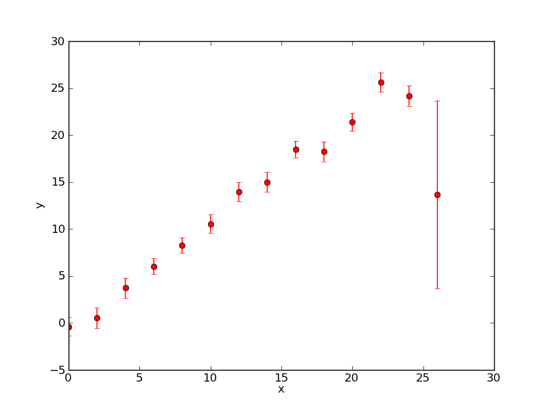
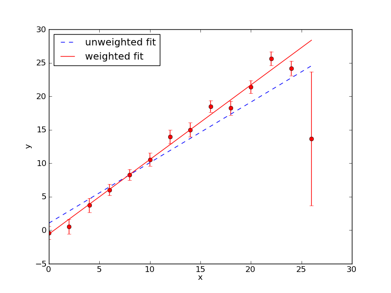
The fit is shown below. The last data point with the large error reduces the slope. It is clear from the other data points that the slope should be steeper. The last data point biases the result. We need a way to weight the data points by their uncertainty so points with a small error will count more than those with a large error. This takes us into the world of maximum likelihood estimation (MLE). The theory of MLE is beyond the scope of this tutorial, but we can use the results. MLE theory tells us that if we have a data set where the errors in the y values are normally distributed then instead of minimizing the function S(a1…aM) we should minimize
 where σy is the uncertainty in the yi data value. This is very similar to the expression for S(a1…aM) except that each data point is wighted by 1/σy2.
 Curve_fit() will automatically minimize χ2 if we pass it the y uncertainties using the optional argument sigma. For example, to fit the data contained in the arrays x and y with y uncertainties in y_err we would use the command curve_fit(func,x,y,sigma=y_err). The plot below shows the fits that result using curve_fit() with and without 1/σy2 weighting. The weighted fit clearly gives a better result.
Exercise 3
Suppose you know that the data in Outlier.txt fits the model y(x) = a + bx. Write a program to use curve_fit() to fit the data weighted by the uncertainties. Use your program to reproduce the plot above. Find the best-fit parameters with and without uncertainty weighting.
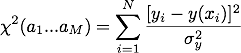
Do I have a good fit?
The fit to Outlier.txt looks like a good fit, but we would like to rely on something more quantitative. Intuitively you might suppose that for a given data point the difference between the data value and the fit value to be of the same order as the uncertainty in that data point |yi - y(xi)|∼ σi. If we divide both sides of this equation by σi, square it, and sum over all the data points, the sum should be approximately equal to N. Using the definition of χ2 we find that χ2 ∼ N. Of course, this doesn't tell the whole story. If we had as many fitting parameters as data points we could always get a perfect fit. (Consider a linear fit with two data points for example.) This suggests that for a good fit χ2 ∼ N - M where M is the number of fitting parameters. Furthermore, if χ2 >> N - M, then either the fitting model is wrong or we have underestimated the uncertainties. On the other hand if χ2 << N - M the fit is too good and you should suspect that we have overestimated the uncertainties.
Hopefully, the argument above seems reasonable, but it isn't very rigorous. A rigorous treatment gives the same result, but is beyond the scope of this tutorial. (For a detailed treatment see Data Reduction and Analysis for the Physical Sciences, 3rd edition by Bevington & Robinson.) A careful derivation requires the assumption that the errors in the data points are normally distributed. In most cases this is a good assumption, but not always. However, if the errors are distributed normally, we can go one step further and compute the probability that, given our data, χ2 would be bigger than N - M by chance. If this probability is small, less than about 0.05, then the values we got from our fit are not likely to represent the data; either our model is wrong or our uncertainties were underestimated. On the other hand, if this probability is nearly 1.0 we might suspect the fit is too good—our uncertainties may have been overestimated.
It's easy to compute χ2 given the data and the fit function by using the sum() function. The probability is more difficult to compute, but as you might expect there is a SciPy function available to do it for you. The needed function is part of the scipy.stats module. This module is a large collection of programs for doing statistical analysis, but we only need the function chi2.cdf(x,dof) where x is χ2 for the fit and dof is the number of degrees of freedom and is equal to N - M. This function actually gives the probability of getting a χ2 value smaller than the value we get from our fit. To get the probability of getting a χ2 larger than our value by chance we have to compute 1.0-chi2.cdf(x,dof). The code below uses curve_fit() to fit the data in Outlier.txt then computes χ2 and probability.
In [123]: x,y,yerr = loadtxt('Outlier.txt',unpack=True)

In [124]: def func(x,a,b):
   .....:     return a + b*x
   .....:

In [125]: from scipy.optimize import curve_fit

In [126]: a_fit,cov = curve_fit(func,x,y,sigma=yerr)

In [127]: chisqr = sum((y-func(x,a_fit[0],a_fit[1]))**2/yerr**2)

In [128]: dof = len(y) - 2

In [129]: from scipy.stats import chi2

In [130]: GOF = 1. - chi2.cdf(chisqr,dof)

In [131]: chisqr
Out[131]: 13.967472760580891

In [132]: dof
Out[132]: 12

In [133]: GOF
Out[133]: 0.30279023555719342
Lines 123 through 126 read the data file and do the fit. Line 127 computes χ2. Line 128 computes the number of degrees of freedom N - M. Line 129 imports the function from scipy.stats that is needed to compute the probability. Line 130 computes the probability which is sometimes called a goodness-of-fit parameter. The last three lines just print the results. We see that the χ2 = 13.9 is close to N - M = 12 as is expected of a good fit. The χ2 per degree of freedom χr2 ≡ χ2/(N - M) is 1.16. This is called the reduced chi squared and should be close to 1.0 for a good fit. The goodness-of-fit parameter in this case is 0.30 which is a reasonable value. We should worry if it is less than about 0.05 or near one.
Exercise 4
The strong nuclear force that binds the nucleons in the nucleus of and atom is mediated by pions. The effective potential energy associated with the nucleon-nucleon interaction is called the Yukawa potential and is given by
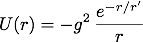 where g is the nuclear force coupling constant, r is the distance between the nucleons, and r' is a constant with dimensions of length. The value of r' is related to the pion mass,
 where m is the mass of the pion, c is the speed of light, and
  is Planck's constant divided by 2π.
Suppose a nuclear physics experiment was able to determine the values for U(r) shown in the table below.
| r (fm) | U (MeV) | σU (MeV) |
|---|---|---|
| 2.9019 | -145.299 | 7.73623 |
| 3.26463 | -111.289 | 8.5017 |
| 3.62737 | -62.1917 | 7.88238 |
| 3.99011 | -46.7048 | 7.46152 |
| 4.35285 | -32.3581 | 8.21121 |
Write a program to determine the values of m and g with uncertainty. Evaluate the quality of the fit. Plot the data with a best fit line. Be careful with units. Report m in MeV/c2 and g in MeV½ fm½.
NOTE: 1 fm = 10-15 m and  = 197.3 MeV fm.