Finding Roots of Equations
Suppose you encounter a system where you need to find the solution to an equation like \(e^x = \cos(x)\). There is clearly no algebraic solution to this equation. The only way to find the value of \(x\) is to do it numerically.
Finding approximate solutions
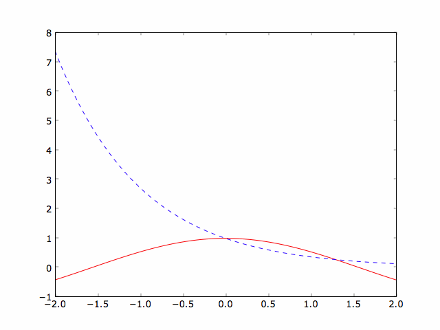
One old-fashioned way to do this is to plot the left-hand-side and the right-hand-side of the relation as a function of \(x\). The values of \(x\) where the two curves intersect are the solutions.
>>> x = linspace(-2,2,100) # create x array
>>> lhs = exp(-x)          # create lhs array
>>> rhs = cos(x)           # create rhs array
>>> plot(x,rhs,'r-')       # plot lhs as solid red curve
>>> plot(x,lhs,'b--')      # plot rhs as dashed blue curve

If you click the figure window active and place the cursor at the points of intersection, the x and y positions of the cursor are displayed in the lower right-hand corner of the window. You can read the approximate solutions from the x-coordinate value. Using this technique I got two solutions; \(x\approx 0\) and 1.3 in the range from -2 to 2.
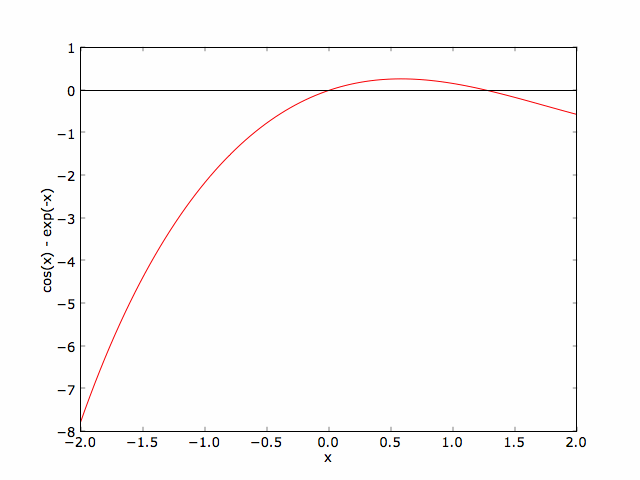
An alternative would to plot the function \(f(x) = \cos(x) - e^x\) and look for the \(x\) values where \(f(x) = 0\). The code and resulting plot is show below. You can get a copy of the code from the downloads page.
"""
plot_function.py
Plots the function cos(x) - exp(-x).
"""

# Import needed modules
from pylab import *

# Define the function
def func(x):
    return cos(x) - exp(-x)

# Create an x-axis and function array
x = linspace(-2,2,100)
y = func(x)

# Plot the result
figure(1)      # define the figure window to use
clf()          # clear the current figure window
plot(x,y,'r-')
xlabel('x')
ylabel('cos(x) - exp(-x)')

# Plot the x-axis to make the zeros easy to find
plot(x,zeros(100),'k-')

This script uses a couple of new plotting commands, figure() and clf(), that weren't covered in the Quick Tour. PyLab allows you to have several plotting windows open at the same time. The figure() command specifies which figure window the following commands will use for the plot. The argument of figure() is an integer specifying the number of the figure window. The clf() command simply clears all the old plot data from the current figure window. To learn more, see the Toolbox Plotting page.
You can zoom in to the relevant part of a plot by clicking the magnifying glass icon at the bottom of the figure window and then selecting the region you want to see up close. This allows you to get a fairly accurate result, but there is a better way that gives a very accurate result. However, its still a good practice to start by plotting the function to find approximate solutions. These approximate solutions are needed to get an acturate solution using the technique described below.
Finding precise solutions
The scipy.optimize module has a built-in function called fsolve(func, x_est) that will give more accurate solutions. This function has two required arguments: func is the name of a function and x_est is the starting estimate for the solution to func(x) = 0. It returns the solution closest to x_est. Like most Scipy functions, fsolve() takes a large number if optional input parameters and can produce more detailed output. To learn more, see the scipy.optimize.fsolve documentation page.
The example below shows an IPython session used to determine more accurate roots of \(f(x)\) in the range from -2 < \(x\) < 2.
In [1]: from pylab import *

In [2]: from scipy.optimize import fsolve

In [3]: def func(x):
   ...:     return cos(x) - exp(-x)
   ...:

In [4]: fsolve(func,0)
Out[4]: 0.0

In [5]: fsolve(func,1.3)
Out[5]: 1.2926957193733983
Exercise 1
The peak of the blackbody spectrum is given by Wien's displacement law
$$\lambda_\mathrm{max} T = C $$
where λmax is the wavelength of the peak of a blackbody, T is it's temperature, and C is a constant. The goal of this exercise is to determine the constant C. We can do this by finding the maximum of the Planck function by taking its derivative with respect to zero and setting it equal to zero. Doing this leads to the equation
$$
\frac{x e^x}{e^x -1} - 5 = 0
$$
where x = hc / λkT, h is the Planck constant, c is the speed of light, and k is the Boltzmann constant. If the solution to the above equation is xmax then λmax T = hc / kxmax so C = hc / kxmax. Follow the procedure above to find approximate value for C, then compute a more accurate value using fsolve().